A time diagram can be used to define the relation between a load and time. The time history analysis using time diagrams is thus dependent on the defined static load.
The time diagrams used in the model are managed in the Time Diagrams dialog box.

Definition Type
Two definition types are available in the list of this section:
- User-defined
- Function
The other sections are adapted to the definition type.
User-Defined
For a user-defined time diagram, you can specify the diagram's properties in a table in the "Times & Multipliers" section.

Enter the "Time" t with the corresponding "Multiplier" k in the table row by row. The order of the rows entered can be arbitrary. This allows you to subsequently add value pairs that lie between the values that have already been defined.
Info
Since there must be a consistent time diagram, the values are displayed in red in case of incorrect order. In this case, use the
![]() button to sort the lines in ascending order.
button to sort the lines in ascending order.

You can delete the selected table row using the
![]() button.
button.
The
![]() button allows you to import the table values of a diagram from Excel. Click the
button allows you to import the table values of a diagram from Excel. Click the
![]() button to export the user-defined time diagram to Excel.
button to export the user-defined time diagram to Excel.
The functions for saving user-defined time diagrams in a library and importing them from there are still under development. The buttons
![]() are thus blocked.
are thus blocked.
If the value pairs have a constant time interval, activate the Δt check box below the table. Then, enter the time step in the text box to the right
![]() . If you now enter multipliers in the table, the time is automatically set with the steps Δt. You can adjust the step Δt at any time in order to enter further value pairs with a different time step. This function is described in the chapter
Accelerograms
.
. If you now enter multipliers in the table, the time is automatically set with the steps Δt. You can adjust the step Δt at any time in order to enter further value pairs with a different time step. This function is described in the chapter
Accelerograms
.
The diagram generated on the basis of the specifications is shown in the lower section. The options for the "Diagram start" and "Diagram end" are described in the Function section.
Function
The second definition type allows you to define the time diagram by any function. The parameter t is reserved for the time in this case.

Enter the function over time in the "Multiplier function" text box. You can use all operators and functions as in the main program (see the chapter Formulas of the RFEM manual). You can also use the global parameters that have been defined for the input in RFEM. Click the
![]() button to open the "Edit Global Parameters" dialog box.
button to open the "Edit Global Parameters" dialog box.
Example of Periodic Function
f(t) = k1 · sin (ω1 · t + φ1) + k2 · sin (ω2 · t + φ2) + ...
The "Time limit" tmax specifies the maximum time for the validity of the function. Changes are applied immediately in the "Multiplier – Time Diagram".
Below the diagram, there are two options for the "Diagram start" and the "Diagram end". They allow you to control which values will be adopted if specifying a longer time in the Time History Analysis Settings or using the Time Slip option for the load case.
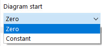
"Zero" means that all values in the negative zone or if t > tmax are set to zero. If you select "Constant", the first or the last diagram value is retained and continued. You can use this option for linear curves to continue the curve with the same inclination, for example.


.png?mw=350&hash=c6c25b135ffd26af9cd48d77813d2ba5853f936c)


![Basic Shapes of Membrane Structures [1]](/en/webimage/009595/2419502/01-en-png-png.png?mw=512&hash=6ca63b32e8ca5da057de21c4f204d41103e6fe20)


.png?mw=512&hash=ea9bf0ab53a4fb0da5c4ed81d32d53360ab2820c)


_1.jpg?mw=350&hash=ab2086621f4e50c8c8fb8f3c211a22bc246e0552)


