Calculation of Concrete Columns Subjected to Combined Bending with RF-CONCRETE Columns

What is combined bending?

Combined bending is designated by the system (M_G0, N) applied in a point C, called the center of pressure. The distance G₀C is called the eccentricity of the external force in relation to the center of gravity G₀ of the pure concrete section.

In combined bending, the value of the bending moment thus depends only on this point, where the reduction of the forces is carried out; here, it is G₀.

The first thing to do in combined bending is to find the position of the center of pressure by calculating e₀.

Considering Geometric Imperfections and Second-Order Effects in ULS

The analysis of elements and structures must take into account the unfavorable effects of any geometric imperfections in the structure, as well as deviations in the position of loads. Deviations in the sections' dimensions are normally taken into account by the partial safety factors for the materials.

Slenderness and Effective Length of Isolated Elements

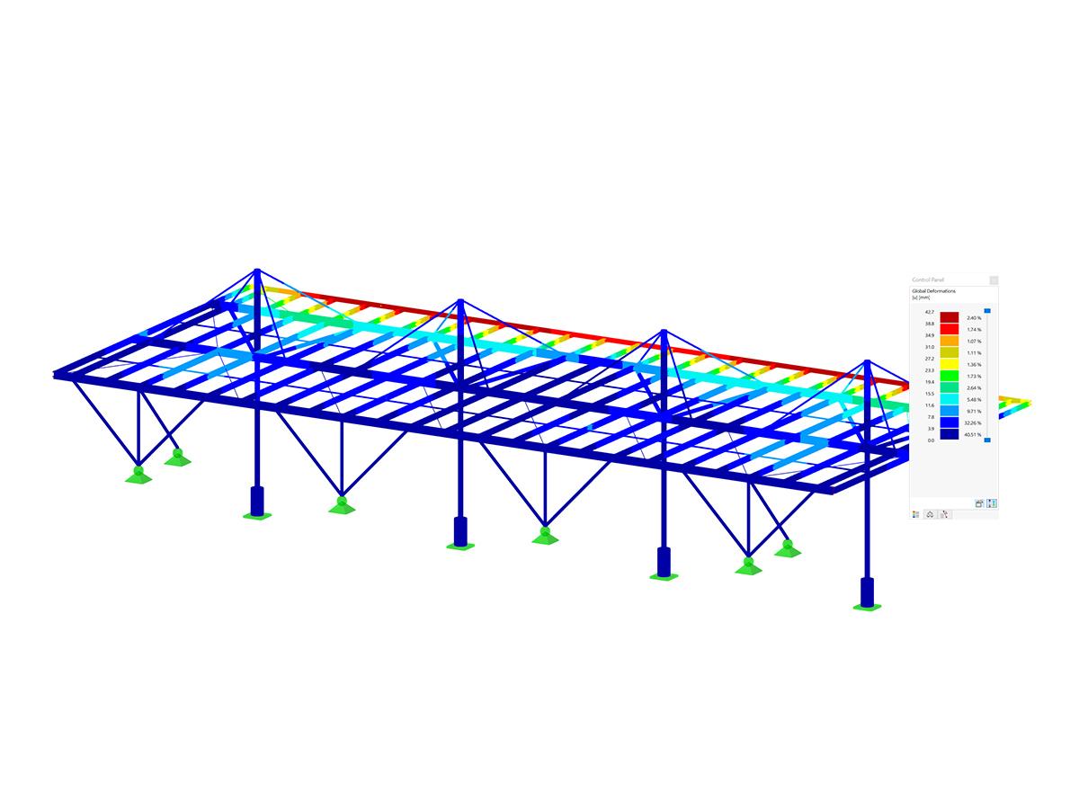
Image 01 shows the possibility in RF-CONCRETE Columns of selecting the buckling length coefficient β by means of modeling the support conditions of isolated elements with constant section and the free length l.

1 Predefined Values of Buckling Length Coefficient Around Y-Axis

Slenderness Criterion for Isolated Elements

It is assumed that second-order effects can be neglected if it is verified that the coefficient of slenderness is lower than the criterion of slenderness.

Considering Creep

The effect of creep must be taken into account in the second-order analysis, considering both the general conditions of creep and the application duration of different loads in a simplified manner by using an effective creep coefficient.

2 Creep Parameters in Input Data

Walls and Isolated Columns of Braced Structures

In the case of isolated elements, the effect of imperfections can be taken into account as eccentricity e_i.

Straight Cross-Sections with Symmetrical Reinforcement

To take into account deviations in the dimensions of cross-sections, the bending moment should be calculated in ULS:

Calculation of Steels Using Interaction Diagrams

The moment-normal force interaction diagrams are charts allowing for the rapid design or verification of straight cross-sections of which the shape and reinforcement distribution are determined in advance. The interaction diagrams are established only for the ultimate limit state. An interaction diagram is drawn using 2 curves constituting a continuous and closed contour called an interaction curve. The course of these curves is based on the equations of the resultant and the resulting moment, depending in particular on the following parameters:

• Concrete and steel deformation diagrams
• Concrete and steel stress diagrams

Thus, for the given cross-section (concrete, reinforcement, position of reinforcing steel), quantities are defined without dimension, based on the design internal forces N_Ed and M_EdG0.

The last equation allows us to determine the necessary reinforcement section by interpolating the curve fields ρ of the interaction diagram, using the reduced orthonormal coordinate system (μ, υ).

Comparison of Theory with RF-CONCRETE Columns Add-on Module

Using a simple example, we compare the results in RF-CONCRETE Columns with the theoretical formulas described previously.

• Loading applied to the center of gravity of pure concrete, of an element of a braced structure:
  • Permanent:
    • N_g = 85 kN
    • M_g = 90 kN.m
  • Varying:
    • N_q = 75 kN
    • M_q = 80 kNm
• Materials:
  • C 25/30 concrete
  • Steel: S 500
• Moment ratio at column base:
  • |M01:| / |M02| = 1/3

• 3D Viewer | Google
• 3D Viewer | Babylon
• Virtual Reality

3 RFEM Model with Modeled Permanent Loads

Material Characteristics

f_cd = 1 ⋅ 25 / 1.5 = 16.67 MPa

f_yd = 500 / 1.15 = 434.78 MPa

Ultimate Limit State

Loading of calculations in ultimate limit state:
M_Ed= 1.35 ⋅ M_g+ 1.5 ⋅ M_q
M_Ed= 1.35 ⋅ 90 + 1.5 ⋅ 80 = 241.50 kNm
N_Ed= 1.35 ⋅ N_g + 1.5 ⋅ N_q
N_Ed= 1.35 ⋅ 85 + 1.5 ⋅ 75 = 227.25 kN

4 Display of Governing Loads

Considering Geometric Imperfections Without Second-Order Effects in ULS

Geometric slenderness for isolated elements, considering the column inserted in a foundation block and restrained by a beam:
l₀ = √2 / 2 ⋅ l = √2 / 2 ⋅ 6.00 = 4.24 m

5 User-Defined Buckling Coefficients in Input Data

Radius of gyration in plane parallel to side h = 55 cm
i_y = h / √12 = 0.55 / √12 = 0.159 m

Radius of gyration in plane parallel to side h = 24 cm
i_z = b / √12 = 0.24 / √12 = 0.069 m

Slendernesses
λ_y = 4.24 / 0.159 = 26.67 m
λ_z = 4.24 / 0.069 = 61.45 m

6 Display of Slenderness Values

Limiting slenderness:
By default, the program takes into account the values according to the effects of creep for A, the initial reinforcements defined in RF-CONCRETE Columns for B, and the ratio of moments at the head and base of the analyzed member for C. However, it is possible to define these values yourself:
A = 0.7
B = 1.1
C = 1.7 - 1 / 3 = 1.37
n = (227.25 ⋅ 10^-3) / (0.24 ⋅ 0.55 ⋅ 16.67) = 0.103
λ_lim = (20 ⋅ 0.7 ⋅ 1.1 ⋅ 1.37) / √(0.103) = 65.74
λ_y< λ_lim ⟹ combined bending calculation in XZ plane
λ_z< λ_lim ⟹ calculation for simple compression in XY plane

7 Display of Slenderness Ratio Limits

The slenderness coefficients being lower than the limit values, it is useless to check the part for buckling, and it is sufficient to have a calculation for combined bending without taking into account the effects of second order, under the following stresses of eccentricity:
e₀ = e₁ + e_i

Eccentricity due to computational loading
e₁ = M_Ed / N_Ed
e₁ : Eccentricity due to computational loading
e₁ = 241.50 / 227.25 = 1.063 m

Loading Corrected for Calculation of Combined Bending

Isolated column from braced structure:
θ₀ = 1 / 200
α_h = 2 / √6 = 0.816
α_m = √0.5 ⋅ (1 + 1 / 1) = 1
θ_i = 0.816 ⋅ 1 / 200 = 0.0041
e_i = 0.0041 ⋅ 4.24 / 2 = 0.0087 m

8 Details of Eccentricity Calculation

Loading applied to the center of gravity of the pure concrete cross-section:

e₀ = e₁+ e_i ≥ Δe₀
e₀ = 1.063 + 0.0087 = 1.072 m

The minimum eccentricity is respected.
M_EdG0 = 227.25 ⋅ 1.072 = 243.61 kNm

9 Displaying Governing Moment Due to Eccentricity

Interaction diagram for a rectangular section with symmetrical reinforcement in combined bending

ν_Ed = (227.25 ⋅ 10^-3) / (0.24 ⋅ 0.55 ⋅ 16.67) = 0.103
μ_Ed = (243.61 ⋅ 10^-3) / (0.24 ⋅ 0.55² ⋅ 16.67) = 0.201

The interaction diagram used to determine the required reinforcement according to the reduced forces ν_Ed, μ_Ed is accessible in the charts of interaction diagrams (Jean Perchat, Traité de béton armé, 3^rd edition of LE MONITEUR, France, 2017).

In the graphical output, the found value is then interpolated between the interaction curves ρ = 0.35 and ρ = 0.40, resulting in ρ = 0.375.
A_s = (0.375 ⋅ 0.24 ⋅ 0.55 ⋅ 16.67) / (434.78) ⋅ 10⁴ = 18.98 cm²

10 Required Reinforcement Determined by RF-CONCRETE Columns

The difference of 0.10 cm² found for the reinforcement comes from the computer's precision on the interpolation of the values of the interaction diagram.

Knowledge Base

KB 001705 | Calculation of Concrete Columns with Combined Loads in RF-CONCRETE Columns

Knowledge Base

KB 001710 | Design of Concrete Columns Subjected to Axial Compression with RF-CONCRETE Members

Knowledge Base

KB 001712 | Design of Concrete Columns Subjected to Axial Compression with RF-CONCRETE Columns